Planimeters from the point of view of a mathematician
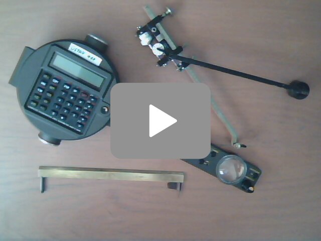
- Click the image on the left to see the video which shows three planimeters in action
- Thanks to Naslouchej mandarinkám for a pleasant music
- Other videos with two funny variants of Prytz planimeter: spoon planimeter and knife planimeter
The purpose of this page:
- a rough information about mechnical devices capable to measure areas and directory to the other resources with detailed explanation or related informations, the main stress is in the mathematics behind as well as in some funny suprising an unusual types of planimeters
- a place for my videos related to planimeters, including planimeters from objects of daily use
- a place for photos and rough information about two unusual planimeters with lack of integration wheel: Prytz planimeter and digital planimeter Ushikata.
According to Wikipedia, planimeter is a measuring instrument used to determine the area of an arbitrary two-dimensional shape. Planimeters have been used by cartographers to find area on map and by scientists to find integral of experimental data (to get mean value, see also here if you understand German).
 There are many types of planimeters. However, only few concepts were
simple and accurate enough in order to attract the attention and be
succesfull and widespread.
There are many types of planimeters. However, only few concepts were
simple and accurate enough in order to attract the attention and be
succesfull and widespread. - This webpage is designed to support the video with presentation of three planimeters of different types.
- The planimeters used in the video as well as planimeters described on this webpage are either property of Department of Forest Management and Applied Geoinformatics (FFWT) or property of people from this department. Several images have been reprinted from an excellent page of Robert L. Foote and http://www.forestry-suppliers.com/
With planimeter we just trace the boundary of a region and obtain the total area of this region. I have found basically three types of planimeters (neglecting other devices of cartographers, some extravagant planimeters and planimeters which were not widesperad):
- Prytz hatchet planimeter,
- linear rolling planimeter and
- Amsler (polar) planimeter and compensating planimeter.
The first planimeter (Prytz) is incredibly simple, but it provides only approximation of the total area. The other two of the planimeters are based on Green's theorem which relates line integral of second kind with double integral (the vector field and the domains of integration are supposed to be sufficiently regular)
$$\oint_{\partial \Omega}P(x,y)\mathrm{d}x +Q(x,y)\mathrm{d}y = \iint_{\Omega} \left(\frac{\partial Q(x,y)}{\partial x}-\frac{\partial P(x,y)}{\partial y}\right)\mathrm{d}x \mathrm{d}y.$$
Prytz hatchet planimeter
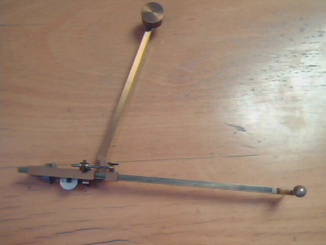
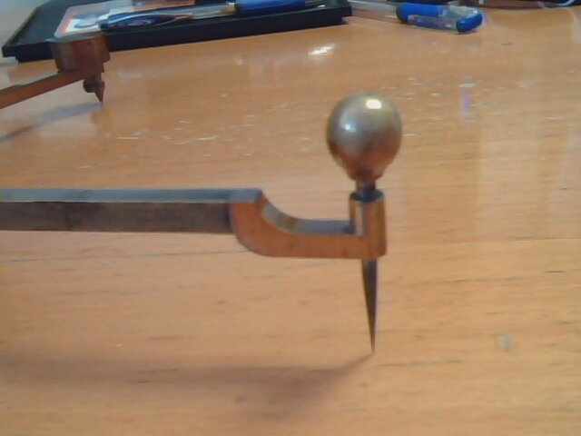
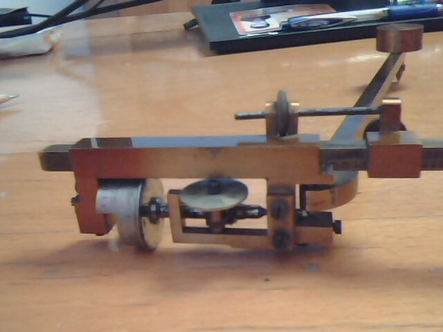
Incredibly simple device. Very rare! Hard to find or buy this planimeter. Perhaps many people do not recognize it as a scientific instrument (looks like strange ruler). Invented about 1894 by Captain Holger Prytz for Danish army.
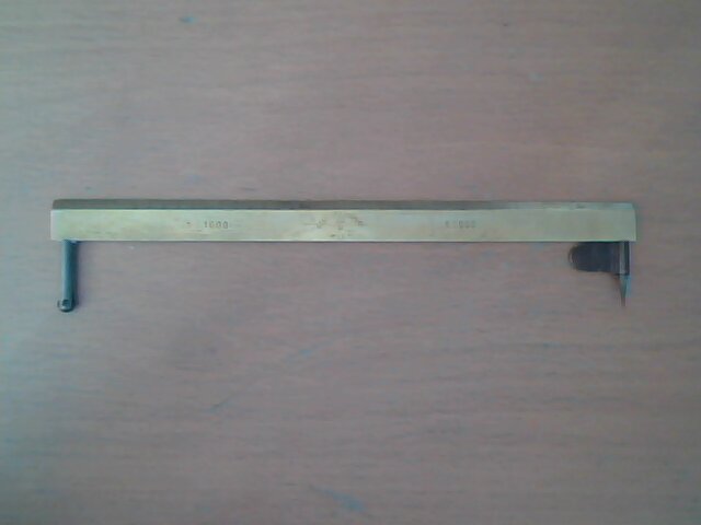
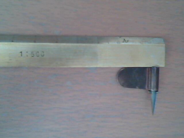
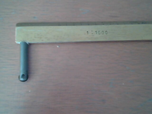
Note that the planimeter on the pictures above has hatchet blade replaced by a sharp wheel and has two scales for maps 1:1000 and 1:500. Another gallery of Prytz planimeters is here. This planimeter can be made at home from wood, wire or coat hanger, rod, lego or replaced by knife, spoon or scooter (I did not test the last possibility yet, but will do and will report in future). There exists a Czech patent which describes how to transform compasses to Prytz planimeter.
Prytz planimeter gives only approximation of the total area, since it includes some principal error. To measure the area with minimal principal error first estimate the position of the center of mass. Then start with the pointer at the center of mass, follow the line to boundary, go around the boundary and using the same line return from the boundary to the center of mass. The second end is displaced by this procedure and the area is approximately equal to the product of the displacement and the length of the planimeter. For the planimeter on the picture, the distance is 20cm, therefore the planimeter should not be used to measure areas with diameter bigger than 10cm and the area is a product of the displacement (in cm) multiplied by 20. The result is in square cm. See also this guide.
Some later authors suggest to make one measurement clockwise, another one counterclockwise and work with the mean value.
Linear (rolling) planimeter
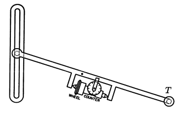
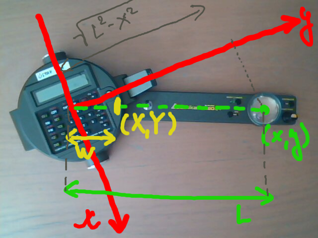
The arm with a perpendicular wheel and tracing point is attached to a cylinder, this cylinder moves along a line. A modern version of this planimeter is on the picture.
There is an excellent mathematical description by Tanya Leise which eplains in details how does the linear planimeter work. Note that in that description there is not written the explicit formula for the direction field which is being integrated by the linear planimeter. This is caused by the fact that as one intermediate step there is shown that some components of the motion have in total zero influece to the final value and it is possible to neglect them. For this reason ve provide alternative explanation of the planimeter, but only very briefly. The interested user should read the material referred above for detailed explanation and then follow mine.
With the coordinate system on picture the tracing arm extends from a point at $y$ axis to the point $(x,y)$ and the vector from one to the second end has coordinates $(x,\sqrt{L^2-x^2})$. Thus the normal unit vector is $$\vec n=\frac 1L\Bigl(-\sqrt{L^2-x^2},x\Bigr).$$ The wheel is perpendicular to the arm, decomposes the motion into the direction tangent and normal the the arm and registers the normal component. As a consequence, the wheel will register just the integral of the normal vector along the curve $C$ which a boundary of region $\Omega$.
Suppose first, for simplicity, that the integration wheel is at the end of the tracing arm, at the point which traces the boundary. Then the integration records integral of the normal vector, i.e. it evaluates the line integral $$I=\oint_{\partial\Omega}\vec n\mathrm{d}\vec r$$ and in cartesian coordinates $$I=\frac 1L \oint_{\partial \Omega} -\sqrt{L^2-x^2}\mathrm{d}x+ x\mathrm{d}y, $$ where $L$ is constant of planimeter (the length of the tracing arm). With application of Green's theorem we get $$I=\frac 1L \iint_{\Omega} \mathrm{d}x\mathrm{d}y$$ and the integral is proportional to the area of $\Omega$, where the proportionality constant is the constat of the planimeter, the length of the tracing arm $L$.
For real planimeter, the integration wheel is in a distance $w<L$ from the end which is fixed to the line. Let $(X,Y)$ be coordinates of the wheel. Thus the integration wheel evaluates $$I=\frac 1L \oint_{\partial \Omega} -\sqrt{L^2-x^2}\mathrm{d}X+ x\mathrm{d}Y. $$ Pure geometry reveals $$ \begin{aligned}X&=\frac wL x\\ Y&=y-\left(1-\frac wL\right)\sqrt{L^2-x^2}.\end{aligned}$$ Differentiating we get $$ \begin{aligned} \mathrm{d}X&=\frac wL \mathrm{d}x\\ \mathrm{d}Y&=\mathrm{d}y+\left(1-\frac wL\right)\frac{x}{\sqrt{L^2-x^2}}\mathrm{d}x.\end{aligned}$$ Substituting into the integral and collecting like terms we get $$\begin{aligned}I&=\frac 1L \oint_{\partial \Omega} \left (-\sqrt{L^2-x^2} \frac wL + \left(1-\frac wL\right)\frac{x^2}{\sqrt{L^2-x^2}} \right )\mathrm{d}x + x\mathrm{d}y \\&=\frac 1L \int_{C} \frac{x^2-Lw}{\sqrt{L^2-x^2}}\mathrm{d}x + x\mathrm{d}y .\end{aligned} $$ and application of Green's theorem reveals the same formula as before: $$I=\frac 1L \iint_{\Omega} \mathrm{d}x\mathrm{d}y.$$
Since the integrated vector field $-{\sqrt{L^2-x^2}}\,\vec{i}+x\,\vec{j}$ is far from trivial even in the simplified case $w=L$, I think that there is no simple explanation for the values which appear on the scale when tracing the boundary. We are interested only in the final number - the total area divided by the length of planimeter.
Amsler's polar planimeter
Invented by Jacob Amsler about 1854. The arm with tracing point and the measuring wheel is attached to the end of another arm. The second end of this arm is fixed to a pole.
You may read a nice story where famous physicist J. C. Maxwell recognised significance of Amsler's planimeter and discarded his own (complicated) planimeter.
The original Amsler concept has been later replaced by compensating planimeter. Polar compensating planimeter does not have attached both arms together and can be assembled in such a way, that the bound of both arms is on one or another side of the line between fixed pole and tracer. To minimize the error of the planimeter (caused by inaccuracy or age of the planimter) you can use both possibilities and consider an average value.
Neglecting the fact that polar coordinates could be natural for this type of problem, let us stay at cartesian coordiantes. We will follow this description. The turning wheel measures $$\frac 1L\oint_{\partial \Omega}(b-y)\mathrm{d}x+(x-a)\mathrm{d}y$$ where $L$ is the length of tracer arm, the fixed pole is at the point $(0,0)$, the end point is at $(x,y)$ and the connection of both arms of planimeter at the point $(a(x,y), b(x,y))$. Really, the end points of the tracing arm are $(a,b)$, and $(x,y)$ which gives vector $(x-a, y-b)$. The normal unit vector (note the length $L$) is $$\vec n=\frac 1L (b-y, x-a)$$ and the integration wheel just catches the motion in this direction (the wheel is perpendicular to the tracing arm). If we put (for simplicity) the integrating wheel to the end point which traces the boundary, then the integration wheel evaluates $$\oint_{\partial \Omega} \vec n \mathrm{d}\vec r$$.
The length of both arms does not change during the process of measuring and thus we have $$a^2+b^2=P^2$$ and $$(x-a)^2+(y-b)^2=L^2,$$ where $P$ is the length of the pole arm of planimeter. From here it can be proved (with a bit of calculations, you have to differentiate both equations of circles with respect to both $x$ and $y$ and solve system of four simultaneous equations) that $$\frac{\partial a}{\partial x}+\frac{\partial b}{\partial y}=1$$ holds if $(a,b)$ and $(x,y)$ are not proportional. Now application of Green's theorem shows $$ \frac 1L\oint_{\partial \Omega}(b-y)\mathrm{d}x+(x-a)\mathrm{d}y= \frac 1L \iint_{\Omega} \left[2-\left(\frac{\partial a}{\partial x}+\frac{\partial b}{\partial y}\right)\right]\mathrm{d}x\mathrm{d}y= \frac 1L\iint_{\Omega} 1\mathrm{d}x\mathrm{d}y= \frac 1L\mathrm{meas}(\Omega). $$
See also this description which is accompanied by the applet showing the vector field.
Note that the above analysis has been done of the integrating whel is at the tracing point. However, in a similar way as for the linear planimeter, it can be shown that the actual position of the wheel on the arm does not matter. Another argument is present in the lecture The Compensating Polar Planimeter by John Eggers. Here it is shown that the value recorded at the wheel is independent on the position of the wheel on the tracing arm. This argument applies also to the linear planimeter
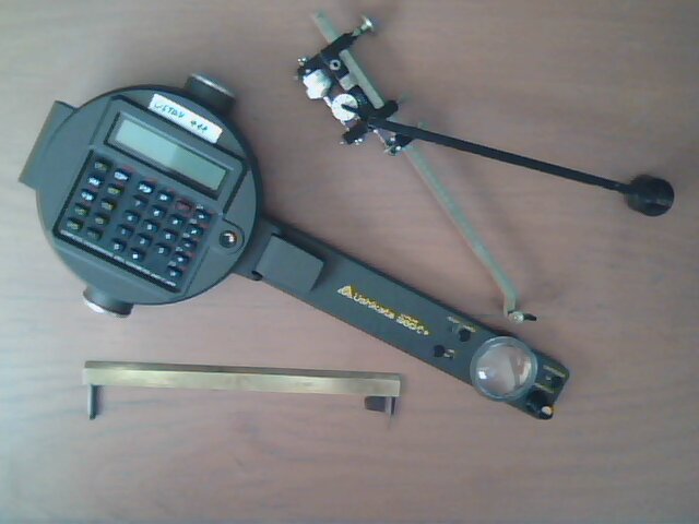
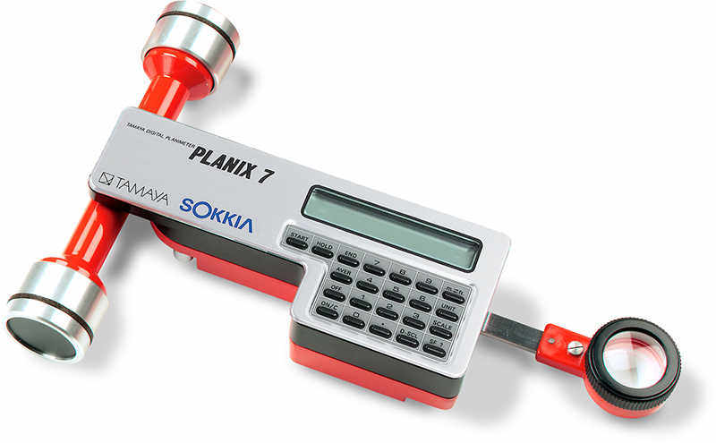
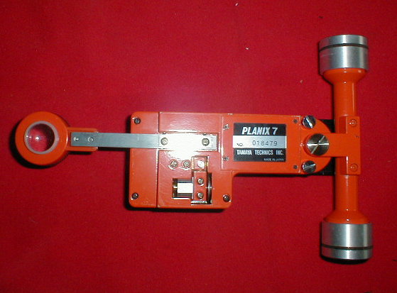
Ushikata digital planimeter
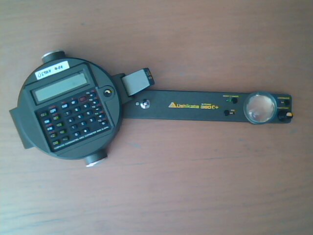
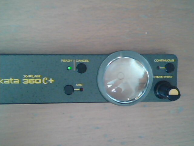
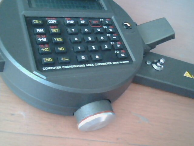
There are digital planimeters which are just digital version of classical devices with integration wheel. Simply the scale is replaced by digital display. From the photos above you can see that Planix 7 planimeters belong to this category. However, the digital planimeter Ushikata presented in the video is based on different idea. It does not have integration wheel and as a consequence, there are no such strong requirements to the perfect flat workplace like for planimeter with integration wheel. See the related patent application for details. How does it work? The idea is simple and (comparing to the planimeters based on Green's theorem) not so interesting from mathematical point of view.
The Ushikata planimeter digital planimeter works on slightly different priciple, described in this and this patents - the integration wheel is missing and a discrete version of Green's theorem is used instead.
The Ushikata planimeter is based on idea to aproximate the boundary by a polyline and thus the region is aproximated by a polygon. The planimeter simply reads in (regular?) intervals the displacement of the measuring arm and the rotation of cylindrical wheels. From these informations computer finds the change of the position of the tracer. This position is used to approximate the next part of boundary by short line. Putting all these short lines together, we approximate region by a polygon. The shoelace formula in the form $$\text{Area}=\frac 12 \sum(x_i+x_{i-1})(y_i-y_{i-1})$$ is used to find the area from vertices coordinates, see the patent application for Device for finding centroid coordinates of figures, which seems to be advanced version of the planimeter above. As clear from this application, another advantage of Ushikata planimeter is that it is capable to calculate lengths of lines, radii of arcs, coordinates of points, moment of inertia and much more.
Final comments
There is also a more elementary theory behind planimeters which is based on pure theory and allows to build one theory for all three types of planimeters (linear, polar and hatchet). I sketched the main ideas here.
Another early device is orthogonal planimeter (cone planimeter). This planimeter is also interesting from mathematical point of view, since it measures directly $\int_a^b f(x)\mathrm{d}x$.
On their website, famous planimeter producer Haff supply a list of around 50 common uses for planimeters. These include botany (area of leaves), medicine (cross-sectional area of organs) and surveying (land areas).
Literature
- Robert L. Foote, Planimeters
- Tanya Leise, Planimeters
- John Eggers, The Compensating Polar Planimeter
Robert Mařík, April 2015, September 2015