Contents

1    Main system

1.1    Notebook

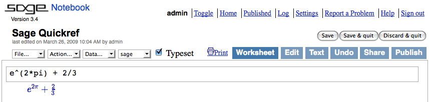
Evaluate cell: \( \displaystyle \langle \) shift-enter\( \displaystyle \rangle \)

Evaluate cell creating new cell: \( \displaystyle \langle \) alt-enter\( \displaystyle \rangle \)

Split cell: \( \displaystyle \langle \) control-;\( \displaystyle \rangle \)

Join cells: \( \displaystyle \langle \) control-backspace\( \displaystyle \rangle \)

Insert math cell: click blue line between cells

Insert text/HTML cell: shift-click blue line between cells

Delete cell: delete content then backspace

1.2    Command line

com\( \displaystyle \langle \) tab\( \displaystyle \rangle \) complete command

*bar*? list command names containing “bar”

command?\( \displaystyle \langle \) tab\( \displaystyle \rangle \) shows documentation

command??\( \displaystyle \langle \) tab\( \displaystyle \rangle \) shows source code

a.\( \displaystyle \langle \) tab\( \displaystyle \rangle \) shows methods for object a    (more: dir(a))

a._\( \displaystyle \langle \) tab\( \displaystyle \rangle \) shows hidden methods for object a    

search_doc("string or regexp")    fulltext search of docs

search_src("string or regexp")    search source code

_ is previous output

1.3    Numbers

Integers: \( \displaystyle \mathbf{Z} =\) ZZ  e.g. -2  -1  0  1  10^100

Rationals: \( \displaystyle \mathbf{Q} =\) QQ  e.g. 1/2  1/1000  314/100  -2/1

Reals: \( \displaystyle \mathbf{R}\approx \) RR  e.g. .5  0.001  3.14  1.23e10000

Polynomials: \( \displaystyle R[x,y]\) e.g. S.<x,y>=QQ[]   x+2*y^3

Interval arithmetic:  RIF  e.g. sage: RIF((1,1.00001))

1.4    Arithmetic

\( \displaystyle ab =\) a*b    \( \displaystyle \frac{a} {b} =\) a/b    \( \displaystyle a^{b} =\) a^b    \( \displaystyle \sqrt{x} =\) sqrt(x)

\( \displaystyle \root{n}\of{x} =\) x^(1/n)    \( \displaystyle |x| =\) abs(x)    \( \displaystyle \log _{b}(x) =\) log(x,b)

Sums: \( \displaystyle \sum _{i=k}^{n}f(i) =\) sum(f(i) for i in (k..n))

Products: \( \displaystyle \mathop{\mathop{∏ }}\nolimits _{i=k}^{n}f(i) =\) prod(f(i) for i in (k..n))

1.5    Builtin constants and functions

Constants: \( \displaystyle \pi =\) pi    \( \displaystyle e =\) e    \( \displaystyle i =\) I = i

\( \displaystyle \infty =\) oo = infinity    NaN=NaN    \( \displaystyle \log (2) =\) log2    

\( \displaystyle \varphi =\) golden_ratio \( \displaystyle \quad γ =\) euler_gamma
   \( \displaystyle 0.915\approx \) catalan    \( \displaystyle 2.685\approx \) khinchin
   \( \displaystyle 0.660\approx \) twinprime    \( \displaystyle 0.261\approx \) merten    \( \displaystyle 1.902\approx \) brun

Approximate: pi.n(digits=18)\( \displaystyle = 3.14159265358979324\)

Builtin functions: sin cos tan sec csc cot sinh  cosh tanh sech csch coth log ln exp ...

2    Symbolic expressions and operations on expressions

2.1    Symbolic expressions

Define new symbolic variables: var("t u v y z")

Symbolic function: e.g. \( \displaystyle f(x) = x^{2}\)  f(x)=x^2

Relations: f==g  f<=g  f>=g  f<g  f>g

_ is previous output

_+a    _-a    _*a    _/a  manipulates equation

Solve \( \displaystyle f(x) = g(x)\) :  solve(f(x)==g(x),x)

solve([f(x,y)==0, g(x,y)==0], x,y)

find_root(f(x), a, b)   find \( \displaystyle x\in [a,b]\) s.t. \( \displaystyle f(x)\approx 0\)

\( \displaystyle \sum _{i=k}^{n}f(i) =\) sum([f(i) for i in [k..n]])

\( \displaystyle \mathop{\mathop{∏ }}\nolimits _{i=k}^{n}f(i) =\) prod([f(i) for i in [k..n]])

2.2    Defining symbolic expressions

Create symbolic variables:
     var("t u theta")  or  var("t,u,theta")

Use * for multiplication and ^ for exponentiation:
\( \displaystyle 2x^{5} + \sqrt{2} =\)  2*x^5 + sqrt(2)

Typeset: show(2*theta^5 + sqrt(2)) \( \displaystyle \mathrel{→}2θ^{5} + \sqrt{2}\)

2.3    Symbolic functions

Symbolic function (can integrate, differentiate, etc.):
  f(a,b,theta) = a + b*theta^2

Also, a “formal” function of theta:
  f = function(’f’,theta)

Piecewise symbolic functions:
Piecewise([[(0,pi/2),sin(1/x)],[(pi/2,pi),x^2+1]])

2.4    Python functions

Defining:

def f(a, b, theta=1):
    c = a + b*theta^2
    return c

Inline functions:

    f = lambda a, b, theta = 1: a + b*theta^2

2.5    Simplifying and expanding

Below \( \displaystyle f\) must be symbolic (so not a Python function):

Simplify: f.simplify_exp(), f.simplify_full(),
f.simplify_log(), f.simplify_radical(),
f.simplify_rational(), f.simplify_trig()

Expand: f.expand(), f.expand_rational()

2.6    Equations

Relations: \( \displaystyle f = g\) : f == g,   \( \displaystyle f\neq g\) : f != g, \( \displaystyle f\leq g\) : f <= g,   \( \displaystyle f\geq g\) : f >= g, \( \displaystyle f < g\) : f < g,   \( \displaystyle f > g\) : f > g

Solve \( \displaystyle f = g\) :  solve(f == g, x),
solve([f == 0, g == 0], x,y)

solve([x^2+y^2==1, (x-1)^2+y^2==1],x,y)

Solutions:   S = solve(x^2+x+1==0, x, solution_dict=True),
    S[0]["x"]   S[1]["x"]   are the solutions

Exact roots: (x^3+2*x+1).roots(x)
Real roots: (x^3+2*x+1).roots(x,ring=RR)
Complex roots: (x^3+2*x+1).roots(x,ring=CC)

2.7    Factorization

Factored form: (x^3-y^3).factor()
List of (factor, exponent) pairs:
(x^3-y^3).factor_list()

3    Calculus

3.1    Limits

\( \displaystyle \lim _{x\to a}f(x) =\) limit(f(x), x=a)

   limit(sin(x)/x, x=0)

\( \displaystyle \lim _{x\to a^{+}}f(x) =\) limit(f(x), x=a, dir=’plus’)

   limit(1/x, x=0, dir=’plus’)

\( \displaystyle \lim _{x\to a^{−}}f(x) =\) limit(f(x), x=a, dir=’minus’)

   limit(1/x, x=0, dir=’minus’)

3.2    Derivatives

\( \displaystyle \frac{d} {dx}(f(x)) =\) diff(f(x),x) = f.diff(x)

\( \displaystyle \frac{\partial\, } {\partial\, x}(f(x,y)) =\) diff(f(x,y),x)

diff \( \displaystyle =\) differentiate \( \displaystyle =\) derivative

   diff(x*y + sin(x^2) + e^(-x), x)

3.3    Integrals

\( \displaystyle \int f(x)dx =\) integral(f,x) = f.integrate(x)

integral(x*cos(x^2), x)

\( \displaystyle \int _{a}^{b}f(x)dx =\) integral(f,x,a,b)

integral(x*cos(x^2), x, 0, sqrt(pi))

\( \displaystyle \int _{a}^{b}f(x)dx\approx \) numerical_integral(f(x),a,b)[0]

   numerical_integral(x*cos(x^2),0,1)[0]

assume(...): use if integration asks a question

   assume(x>0)

3.4    Taylor and partial fraction expansion

Taylor polynomial, deg \( \displaystyle n\) about \( \displaystyle a\) :
taylor(f,x,a,n)\( \displaystyle \approx c_{0} + c_{1}(x − a) +\cdots +c_{n}(x − a)^{n}\)

  taylor(sqrt(x+1), x, 0, 5)

Partial fraction:

  (x^2/(x+1)^3).partial_fraction()

3.5    Numerical roots and optimization

Numerical root: f.find_root(a, b, x)
  (x^2 - 2).find_root(1,2,x)
Maximize: find \( \displaystyle (m,x_{0})\) with \( \displaystyle f(x_{0}) = m\) maximal
  f.find_maximum_on_interval(a, b, x)
Minimize: find \( \displaystyle (m,x_{0})\) with \( \displaystyle f(x_{0}) = m\) minimal
  f.find_minimum_on_interval(a, b, x)

Minimization: minimize(f, start_point)
   minimize(x^2+x*y^3+(1-z)^2-1, [1,1,1])

3.6    Multivariable calculus

Gradient: f.gradient() or f.gradient(vars)
    (x^2+y^2).gradient([x,y])

Hessian: f.hessian()
    (x^2+y^2).hessian()

Jacobian matrix: jacobian(f, vars)
    jacobian(x^2 - 2*x*y, (x,y))

4    Graphics

4.1    2D graphics

line([(\( \displaystyle x_{1}\) ,\( \displaystyle y_{1}\) ),\( \displaystyle \mathop{\mathop{…}}\) ,(\( \displaystyle x_{n}\) ,\( \displaystyle y_{n}\) )],\( \displaystyle options\) )

polygon([(\( \displaystyle x_{1}\) ,\( \displaystyle y_{1}\) ),\( \displaystyle \mathop{\mathop{…}}\) ,(\( \displaystyle x_{n}\) ,\( \displaystyle y_{n}\) )],\( \displaystyle options\) )

circle((\( \displaystyle x\) ,\( \displaystyle y\) ),\( \displaystyle r\) ,\( \displaystyle options\) )

text("txt",(\( \displaystyle x\) ,\( \displaystyle y\) ),\( \displaystyle options\) )

options as in plot.options, e.g. thickness=\( \displaystyle pixel\) ,

rgbcolor=(\( \displaystyle r\) ,\( \displaystyle g\) ,\( \displaystyle b\) ),    hue=\( \displaystyle h\)    where \( \displaystyle 0 ≤ r,b,g,h ≤ 1\)

show(graphic, options)

use figsize=[w,h] to adjust size

use aspect_ratio=number to adjust aspect ratio

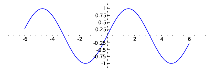
plot(f(\( \displaystyle x\) ),\( \displaystyle (x,x_{min},x_{max})\) ,\( \displaystyle options\) )

parametric_plot((f(\( \displaystyle t\) ),g(\( \displaystyle t\) )),\( \displaystyle (t,t_{min},t_{max})\) ,\( \displaystyle options\) )

polar_plot(f(\( \displaystyle t\) ),\( \displaystyle (t,t_{min},t_{max})\) ,\( \displaystyle options\) )

combine: circle((1,1),1)+line([(0,0),(2,2)])

animate(list of graphics, options).show(delay=20)

4.2    3D graphics

line3d([(\( \displaystyle x_{1}\) ,\( \displaystyle y_{1}\) ,\( \displaystyle z_{1}\) ),\( \displaystyle \mathop{\mathop{…}}\) ,(\( \displaystyle x_{n}\) ,\( \displaystyle y_{n}\) ,\( \displaystyle z_{n}\) )],\( \displaystyle options\) )

sphere((\( \displaystyle x\) ,\( \displaystyle y\) ,\( \displaystyle z\) ),\( \displaystyle r\) ,\( \displaystyle options\) )

text3d("txt", (\( \displaystyle x\) ,\( \displaystyle y\) ,\( \displaystyle z\) ), \( \displaystyle options\) )

tetrahedron((\( \displaystyle x\) ,\( \displaystyle y\) ,\( \displaystyle z\) ),\( \displaystyle size\) ,\( \displaystyle options\) )

cube((\( \displaystyle x\) ,\( \displaystyle y\) ,\( \displaystyle z\) ),\( \displaystyle size\) ,\( \displaystyle options\) )

octahedron((\( \displaystyle x\) ,\( \displaystyle y\) ,\( \displaystyle z\) ),\( \displaystyle size\) ,\( \displaystyle options\) )

dodecahedron((\( \displaystyle x\) ,\( \displaystyle y\) ,\( \displaystyle z\) ),\( \displaystyle size\) ,\( \displaystyle options\) )

icosahedron((\( \displaystyle x\) ,\( \displaystyle y\) ,\( \displaystyle z\) ),\( \displaystyle size\) ,\( \displaystyle options\) )

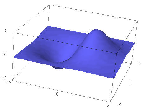
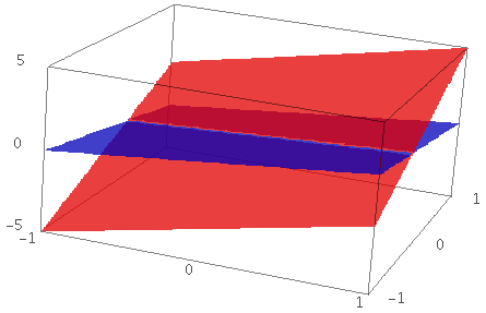
plot3d(f(\( \displaystyle x,y\) ),\( \displaystyle (x,x_{b},x_{e})\) , \( \displaystyle (y,y_{b},y_{e})\) ,\( \displaystyle options\) )

parametric_plot3d((f,g,h),\( \displaystyle (t,t_{b},t_{e})\) ,\( \displaystyle options\) )

parametric_plot3d((f(\( \displaystyle u,v\) ),g(\( \displaystyle u,v\) ),h(\( \displaystyle u,v\) )),

\( \displaystyle (u,u_{b},u_{e})\) ,\( \displaystyle (v,v_{b},v_{e})\) ,\( \displaystyle options\) )

options: aspect_ratio=\( \displaystyle [1,1,1]\) , color="red"

opacity=0.5, figsize=6, viewer="tachyon"

5    Matrices

5.1    Basic matrix algebra

\( \displaystyle \left (\array{ 1\cr 2} \right ) =\) vector([1,2])

\( \displaystyle \left (\array{ 1& 2\cr 3& 4} \right ) =\) matrix(QQ,[[1,2],[3,4]], sparse=False)

\( \displaystyle \left (\array{ 1& 2& 3\cr 4& 5 & 6} \right ) =\) matrix(QQ,2,3,[1,2,3, 4,5,6])

\( \displaystyle \left |\array{ 1& 2\cr 3& 4} \right | =\) det(matrix(QQ,[[1,2],[3,4]]))

\( \displaystyle Av =\) A*v    \( \displaystyle A^{−1} =\) A^-1    \( \displaystyle A^{t} =\) A.transpose()

Solve \( \displaystyle Ax = v\) :  A\v   or  A.solve_right(v)

Solve \( \displaystyle xA = v\) :  A.solve_left(v)

Reduced row echelon form:  A.echelon_form()

Rank and nullity: A.rank()    A.nullity()

Hessenberg form: A.hessenberg_form()

Characteristic polynomial: A.charpoly()

Eigenvalues: A.eigenvalues()

Eigenvectors: A.eigenvectors_right() (also left)

Gram-Schmidt: A.gram_schmidt()

Visualize: A.plot()

LLL reduction: matrix(ZZ,...).LLL()

Hermite form: matrix(ZZ,...).hermite_form()

5.2    Matrix Constructions

Caution: Row, column numbering begins at 0
A = matrix(ZZ, [[1,2],[3,4],[5,6]])
  \( \displaystyle 3\times 2\) over the integers
B = matrix(QQ, 2, [1,2,3,4,5,6])
  2 rows from a list, so \( \displaystyle 2\times 3\) over rationals
C = matrix(CDF, 2, 2, [[5*I, 4*I], [I, 6]])
  complex entries, 53-bit precision
Z = matrix(QQ, 2, 2, 0) zero matrix
D = matrix(QQ, 2, 2, 8)
  diagonal entries all \( \displaystyle 8\) , other entries zero
I = identity_matrix(5)\( \displaystyle 5\times 5\) identity matrix
J = jordan_block(-2,3)
  \( \displaystyle 3\times 3\) matrix, \( \displaystyle − 2\) on diagonal, \( \displaystyle 1\) ’s on super-diagonal var(’x y z’); K = matrix(SR, [[x,y+z],[0,x^2*z]])
  symbolic expressions live in the ring SR
L=matrix(ZZ, 20, 80, {(5,9):30, (15,77):-6})
  \( \displaystyle 20\times 80\) , two non-zero entries, sparse representation

5.3    Matrix Multiplication

u = vector(QQ, [1,2,3]),   v = vector(QQ, [1,2])
A = matrix(QQ, [[1,2,3],[4,5,6]])
B = matrix(QQ, [[1,2],[3,4]])
u*A,   A*v,   B*A,   B^6,   B^(-3) all possible
B.iterates(v, 6) produces \( \displaystyle vB^{0},vB^{1},\mathop{\mathop{…}},vB^{5}\)
  rows = False moves v to right of matrix powers
f(x)=x^2+5*x+3 then f(B) is possible
B.exp() matrix exponential, i.e. \( \displaystyle \sum _{k=0}^{\infty }\frac{B^{k}} {k!} \)

5.4    Matrix Spaces

M = MatrixSpace(QQ, 3, 4)
  dimension 12 space of \( \displaystyle 3\times 4\) matrices
A = M([1,2,3,4,5,6,7,8,9,10,11,12])
  is a \( \displaystyle 3\times 4\) matrix, an element of M
M.basis()
M.dimension()
M.zero_matrix()

5.5    Matrix Operations

5*A+2*B linear combination
A.inverse(), also A^(-1), ~A
  ZeroDivisionError if singular
A.transpose()
A.antitranspose() transpose + reverse orderings
A.adjoint() matrix of cofactors
A.conjugate() entry-by-entry complex conjugates
A.restrict(V) restriction on invariant subspace V

5.6    Row Operations

Row Operations: (change matrix in place)
Caution: first row is numbered 0
A.rescale_row(i,a) a*(row i)
A.add_multiple_of_row(i,j,a) a*(row j) + row i
A.swap_rows(i,j)
Each has a column variant, row\( \displaystyle →\) col
For a new matrix, use e.g. B = A.with_rescaled_row(i,a)

5.7    Echelon Form

A.echelon_form(), A.echelonize(), A.hermite_form()
Caution: Base ring affects results
A = matrix(ZZ,[[4,2,1],[6,3,2]])
B = matrix(QQ,[[4,2,1],[6,3,2]])

A.pivots() indices of columns spanning column space
A.pivot_rows() indices of rows spanning row space

5.8    Pieces of Matrices

Caution: row, column numbering begins at 0
A.nrows()
A.ncols()
A[i,j] entry in row i and column j
  Caution: OK: A[2,3] = 8, Error: A[2][3] = 8
A[i] row i as immutable Python tuple
A.row(i) returns row i as Sage vector
A.column(j) returns column j as Sage vector
A.list() returns single Python list, row-major order
A.matrix_from_columns([8,2,8])
  new matrix from columns in list, repeats OK
A.matrix_from_rows([2,5,1])
  new matrix from rows in list, out-of-order OK
A.matrix_from_rows_and_columns([2,4,2],[3,1])
  common to the rows and the columns
A.rows() all rows as a list of tuples
A.columns() all columns as a list of tuples
A.submatrix(i,j,nr,nc)
  start at entry (i,j), use nr rows, nc cols
A[2:4,1:7], A[0:8:2,3::-1] Python-style list slicing

5.9    Combining Matrices

A.augment(B) A in first columns, B to the right
A.stack(B) A in top rows, B below
A.block_sum(B) Diagonal, A upper left, B lower right
A.tensor_product(B) Multiples of B, arranged as in A

5.10    Scalar Functions on Matrices

A.rank()
A.nullity() == A.left_nullity()
A.right_nullity()
A.determinant() == A.det()
A.permanent()
A.trace()
A.norm() == A.norm(2) Euclidean norm
A.norm(1) largest column sum
A.norm(Infinity) largest row sum
A.norm(’frob’) Frobenius norm

5.11    MatrixProperties

.is_zero() (totally?), .is_one() (identity matrix?),
.is_scalar() (multiple of identity?), .is_square(),
.is_symmetric(), .is_invertible(), .is_nilpotent()

5.12    Eigenvalues

A.charpoly(’t’) no variable specified defaults to x
  A.characteristic_polynomial() == A.charpoly()
A.fcp(’t’) factored characteristic polynomial
A.minpoly() the minimum polynomial
  A.minimal_polynomial() == A.minpoly()
A.eigenvalues() unsorted list, with mutiplicities
A.eigenvectors_left() vectors on left, _right too
  Returns a list of triples, one per eigenvalue:
    e: the eigenvalue
    V: list of vectors, basis for eigenspace
    n: algebraic multiplicity
A.eigenmatrix_right() vectors on right, _left too
  Returns two matrices:
    D: diagonal matrix with eigenvalues
    P: eigenvectors as columns (rows for left version)
      has zero columns if matrix not diagonalizable

5.13    Solutions to Systems

A.solve_right(B) _left too
  is solution to A*X = B, where X is a vector or matrix
A = matrix(QQ, [[1,2],[3,4]])
b = vector(QQ, [3,4])
  then A\b returns the solution (-2, 5/2)

6    Linear algebra

Vector space \( \displaystyle K^{n} =\)  K^n  e.g.  QQ^3   RR^2   CC^4

Subspace: span(vectors, field )

E.g., span([[1,2,3], [2,3,5]], QQ)

Kernel: A.right_kernel() (also left)

Sum and intersection: V + W  and  V.intersection(W)

Basis: V.basis()

Basis matrix: V.basis_matrix()

Restrict matrix to subspace: A.restrict(V)

Vector in terms of basis: V.coordinates(vector)

6.1    Vector Constructions

Caution: First entry of a vector is numbered 0
u = vector(QQ, [1, 3/2, -1]) length 3 over rationals
v = vector(QQ, {2:4, 95:4, 210:0})
  211 entries, nonzero in entry 4 and entry 95, sparse

6.2    Vector Operations

u = vector(QQ, [1, 3/2, -1])
v = vector(ZZ, [1, 8, -2])
2*u - 3*v linear combination
u.dot_product(v)
u.cross_product(v) order: u\( \displaystyle \times \) v
u.inner_product(v) inner product matrix from parent
u.pairwise_product(v) vector as a result
u.norm() == u.norm(2) Euclidean norm
u.norm(1) sum of entries
u.norm(Infinity) maximum entry
A.gram_schmidt() converts the rows of matrix A

6.3    Vector Spaces

U = VectorSpace(QQ, 4) dimension 4, rationals as field
V = VectorSpace(RR, 4) “field” is 53-bit precision reals
W = VectorSpace(RealField(200), 4)
  “field” has 200 bit precision
X = CC^4 4-dimensional, 53-bit precision complexes
Y = VectorSpace(GF(7), 4) finite
  Y.finite() returns True
  len(Y.list()) returns \( \displaystyle 7^{4} = 2401\) elements

6.4    Vector Space Properties

V.dimension()
V.basis()
V.echelonized_basis()
V.has_user_basis() with non-canonical basis?
V.is_subspace(W) True if W is a subspace of V
V.is_full() rank equals degree (as module)?
Y = GF(7)^4,   T = Y.subspaces(2)
  T is a generator object for 2-D subspaces of Y
  [U for U in T] is list of 2850 2-D subspaces of Y

6.5    Constructing Subspaces

span([v1,v2,v3], QQ) span of list of vectors over ring

For a matrix A, objects returned are
  vector spaces when base ring is a field
  modules when base ring is just a ring
A.left_kernel() == A.kernel() right_ too
A.row_space() == A.row_module()
A.column_space() == A.column_module()
A.eigenspaces_right() vectors on right, _left too
  Pairs, having eigenvalue with its right eigenspace

If V and W are subspaces
V.quotient(W) quotient of V by subspace W
V.intersection(W) intersection of V and W
V.direct_sum(W) direct sum of V and W
V.subspace([v1,v2,v3]) specify basis vectors in a list

6.6    Dense versus Sparse

Note: Algorithms may depend on representation
Vectors and matrices have two representations
  Dense: lists, and lists of lists
  Sparse: Python dictionaries
.is_dense(), .is_sparse() to check
A.sparse_matrix() returns sparse version of A
A.dense_rows() returns dense row vectors of A
Some commands have boolean sparse keyword

6.7    Rings

Note: Many algorithms depend on the base ring
<object>.base_ring(R) for vectors, matrices,…
  to determine the ring in use
<object>.change_ring(R) for vectors, matrices,…
  to change to the ring (or field), R,
R.is_ring(),   R.is_field()
R.is_integral_domain(),   R.is_exact()

Some ring and fields
  ZZ   integers, ring
  QQ   rationals, field
  QQbar   algebraic field, exact
  RDF   real double field, inexact
  RR   53-bit reals, inexact
  RealField(400)   400-bit reals, inexact
  CDF,   CC,   ComplexField(400)   complexes, too
  RIF   real interval field
  GF(2)   mod 2, field, specialized implementations
  GF(p) == FiniteField(p)   p prime, field
  Integers(6)   integers mod 6, ring only
  CyclotomicField(7)   rationals with 7\( \displaystyle ^{th}\) root of unity
  QuadraticField(-5, ’x’)   rationals adjoin x=\( \displaystyle \sqrt{−5}\)
  SR   ring of symbolic expressions

6.8    Vector Spaces versus Modules

A module is “like” a vector space over a ring, not a field
Many commands above apply to modules
Some “vectors” are really module elements

7    Specials

7.1    Python modules

import module_name

module_name.\( \displaystyle \langle \) tab\( \displaystyle \rangle \) and help(module_name)

7.2    Profiling and debugging

time command:    show timing information

timeit("command"): accurately time command

t = cputime(); cputime(t): elapsed CPU time

t = walltime(); walltime(t): elapsed wall time

%pdb: turn on interactive debugger (command line only)

%prun command: profile command (command line only)